ORCS
An Oblivious Routing Congestion Simulator
Introduction
Bisection Bandwidth
In the following Network topology boxes symbolize switches while circles resemble hosts.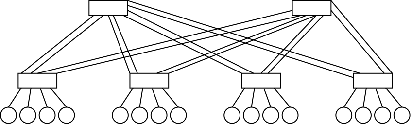
Such a network is said to have full bisection bandwidth (FBB) because, no matter how we partition the sixteen nodes in two sets of equal size, there are always eight cables going from one set to the other. At the same time there can not be more than eight nodes in one of the two sets, otherwise they would not be of equal size. So if we imagine that all hosts in one partition send data to a host in the other partition in such a way that each host has exactly one communication partner, we can assume that we get eight times the bandwidth of a single link, since we can utilize eight links for our data transfer.
Usually network topologies for high performance computing (HPC) systems are evaluated by their bisection bandwidth, since the bisection bandwidth of a network tells us how much data can be send through the network. Since the bisection bandwidth is defined as the bandwidth for the worst case partitioning, it is intended to give a lower bound for the available bandwidth.
Static routing
Many HPC interconnection networks, such as InfiniBand, use static routing. This means that the path that a packet from Host A will take to reach Host B is determined at some point and not changed afterwards, even if other host pairs use the same path at the same time. For InfiniBand the routing is destination based, which means that if a packet is currently at a certain host or switch, the rest of it's path is determined only by it's destination. This approach has advantages when building switches. If a packet arrives at a switch, the switch only has to inspect the destination of the packet to decide through which port it will leave the switch. So every switch has a simple table with all hosts he has to forward traffic to and the port through which each host is reached. This table is called Linear Forwarding Table (LFT) in InfiniBand terminology. So what's the problem with static routing? We use the same network as before, but now we added routing information. The hosts are numbered from 1 to 16. The small numbers next to the cables show for which destination this cable is used. Note that there are two different pairs of numbers on every cable (red and green), one group for each direction.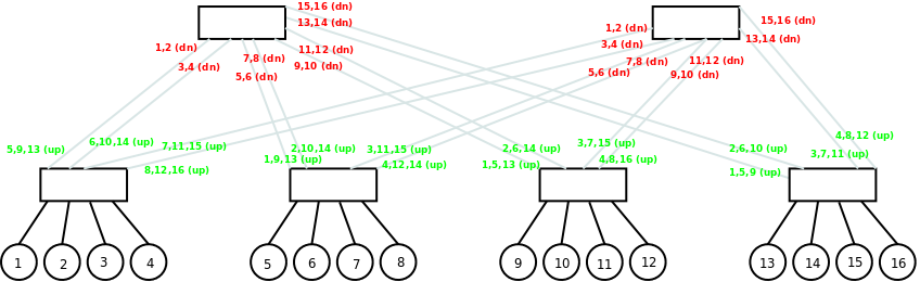
Congestion
Our example network allows us to create some bisection traffic patterns that have full bandwidth, such as (1,5),(2,6),(3,7),(4,8),(9,13),(10,14),(11,15),(12,16). But other bisection patterns show a different behaviour. For example in the pattern (1,5),(2,9),(3,13),(4,6),(7,8),(10,11),(12,14),(15,16) the connections (1,5),(2,9) and (3,13) have all share the same cable. Therefore, theoretically, only one third of the link bandwidth is available to these connections, due to congestion. Note that links are full-duplex for most HPC interconnection networks, so messages can travel in both directions simultaneously without interference. The effect of congestion on latency and bandwidth in an InfiniBand network is shown in the graphs below.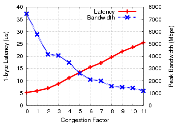
Simulation
To evaluate the communication performance of a statically routed network theoretical metrics such as Bisection Bandwidth are not sufficient. Bisection Bandwidth in particular does neither provide an upper nor a lower bound for the bandwidth available to applications: If we assume the mapping of processes to hosts in a network is completely random, an application that communicates in a bisection-scheme could be mapped to a network such that there are much more links available than in the worst case partitioning used by the bisection bandwidth metric. In this case bisection bandwidth underestimates the network performance. On the other hand, if the application is mapped such that the available links between both partitions matches the amount of links in the worst case partitioning, it is possible that, for the used communication pattern, not all links are utilized due to the static routing tables, as shown in the example above.To be able to study the influence of congestion on the performance of InfiniBand networks, we developed ORCS, the Oblivious Routing Congestion Simulator. It is capable of simulating a variety of communication patterns on staticly routed networks. The network topology input files can be constructed by querying InfiniBand installations with tools that come with the InfiniBand software stack OFED. Given a network topology with routing information and the traffic pattern you want to simulate on this network, ORCS performs a user-specified number of simulation runs. In each run it randomly maps the communicating processes to the available hosts in the network and calculates the congestion factor for every link in the network. After all simulations are completed ORCS analyses the congestion factors to produce the final result according to one of the predefined metrics.
The current version of our Simulator uses a very simple communication model: messages are of uniform length and communication patterns consist of multiple rounds, where all communication in one round happens simultaneously, while communication in different rounds does not interfere with each other. Due to its simplicity it is easy to parallelize ORCS and run simulations on big network topologies. We can simulate networks with more than 20.000 hosts.
Usage
Input File Format
The network topology for the simulated network is given to the simulator as a directed graph in the dot format. An example for a network topology graph in the dot format is given in the file example.dot. Our simulator differentiates between two types of nodes: hosts and switches. All nodes that have a name starting with the letter "H" are recognized as hosts, all other nodes are regarded as switches. As shown in the example, not only the network topology is described in the dot file but it also contains routing information. An edge in a dot graph can have arbitrary information attached. We add the routing information in comments along these edges. For example the definition for the edge between S11 and S1 in the example input file contains the comment string ''H1,H2'': this means that packets that have been routed to S11 are supposed to take this edge to reach the next hop if and only if their final destination is one of the hosts H1 or H2. Hosts are connected to exactly one switch with one physical link. That means that all traffic emitted by a host has to use the respective edge in the network graph since there is no other way to leave the host. In that case all hosts (except the sending one) would have to be listed in the comment string for such edges. This would lead to unnecessarily large files, therefore we introduced the ''*'' character which matches any host in the network.Building the Simulator
To build the simulator and all the related tools, execute theinstall.sh script from the ORCS tarball. Note that you have to
have the Boost
Graph Library and the GNU Scientific Library installed
to build the simulator. Other tools that come with our simulator need SWIG.
Obtaining Input Files from InfiniBand Networks
Writing such files by hand is tiresome and error prone. Luckily the InfiniBand software stack provides tools to extract all the needed information from a working network installation. These tools,ibdiagnet and
ibnetdiscover, can be used in conjunction with the
get_network_graph script in our simulator package. An example
session to illustrate the usage of these tools is given below. # ibdiagnet -v -o .# ibnetdiscover -s > ibndisc.out$ get_network_graph ibdiagnet.fdbs ibndisc.out > topo.dotNote that ibdiagnet and ibnetdiscover have to be executed with superuser privileges. Both tools are part of the OFED software package. The ibdiagnet tool will write a variety of output files named ibdiagnet.* into the current working directory, where ibnetdiscover writes to stdout and therefore its output was redirected to a file called ibndisc.out. Our conversion script has to be called with two command line arguments, the ibdiagnet fdbs output file and the ibnetdiscover output file. The resulting dot graph is written to stdout and should be redirected into a file.
Running Simulations
In this section we will give a short overview over the most important features of our simulator and how to use them. If you start the simulator with the example.dot input file given above:./orcs -i example.dot
it will perform one simulation bisection communication pattern, where one half of the nodes are senders and the other half are receivers. Each sender transmits data to exactly one receiver while each receiver gets data from exactly one sender. You can change the pattern with the
-p
pattern
or --ptrn pattern option. The available patterns
are described below. The number of simulation iterations can be changed by the
-n number or --num_runs number option. The output for
the simulation show above could look like this:
Input File: example.dot[...]weight 1: 4 of the 8 connections (50.00%)weight 2: 4 of the 8 connections (50.00%)BW: 0.750000The omitted part only contains information about the parameters for the simulation run, which is useful for analyzing an output file.
In this simulation run eight data transmissions took place, of which four where uncongested and four had to share at least one link on there route with another data transfer and therefore only provided half of the bandwidth for each of these transmissions. Overall the application experienced 75% of the peak bandwidth (all data transfers are uncongested).
If you re-run the simulation a couple of times you will notice that the result is not always the same. Sometimes you might even get peak bandwidth with this example. This shows that
Available Communication Patterns
In the following we will explain the predefined communication patterns that the user can select for simulations. For a complete definition of each pattern please consult the Technical Report on our simulator, which can be found in the References section. The pattern is selected with the-p, --ptrn=STRING command line option. Valid
parameters are: rand, null, bisect, bisect_fb_sym, tree, bruck, gather,
scatter, ring, recdbl, 2neighbor, 4neighbor, 6neighbor and ptrnvsptrn.
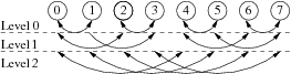
The communication patterns for our simulators can have multiple levels. Each level is simulated independently, data transmissions in one level do not influence transmissions in other levels. Each level is defined as a set of sender and receiver pairs, all data transmissions defined in one level will happen in parallel and all messages in our simulation ara communication pattern can be defines as a list of sets of sender-receiver pairs, for example the pattern [{(0,1), (2,3)}, {(1,0), (3,2)}] describes a communication between four nodes which has two levels. In level 0 two nodes send a message two the other two nodes, in level 1 data is sent in the opposite direction. Note that the numbers in the communication pattern do not correspond to any particular node in the network topology input file. The mapping of nodes in the communication pattern to hosts in the network is done randomly before every simulation iteration.
The rand pattern: in this communication pattern every node sends a single data stream to one randomly selected node and receives a single data stream from one randomly selected node.
The null pattern: this communication pattern is only useful in conjunction with the ptrnvsptrn communication pattern. In the null pattern no communication happens.
The bisect pattern splits the hosts in the network in equally sized halves. Each node in the first half sends a data stream to a node in the second half. If the number of hosts in the network is odd we can not form equal sized partitions, therefore, one host is ignored.
The bisect_fb_sym is similar to the bisect pattern described before. While the flow of data was unidirectional in that pattern because there was a ''sender'' and a ''receiver'' partition, traffic is send in both directions in this pattern.
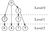
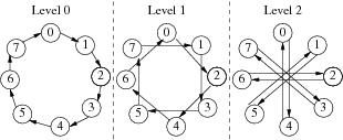
The tree pattern simulates a binomial tree. An example of a binomial tree with eight nodes is shown below:
The bruck pattern simulates a pattern where each node is sending and receiving a message in every one of the log[2](n) levels the pattern consists of, where n is the communicator size. An example of a bruck pattern with eight nodes is shown below:
In the gather pattern a single node receives a message from all other nodes in the communicator. This pattern consists of a single level.
The scatter pattern is very similar to the gather pattern described before, this time a single node sends a message to all other nodes in the communicator. All communication happens in one level.
The ring pattern describes a communication scheme where one node sends a message to another node, this node passes the data to the next node which has not participated in the communication yet, and so on, until all nodes received a message. In the last step the node which received the data most recently sends a message to the node which started the communication and thereby closes the ring. Because of the dependencies (we assume node k can not send the data before it received the message from node k-1), each data transfer occurs in a single level. That means this pattern can never generate congestion by itself, but it is still useful in conjunction with the ptrnvsptrn pattern which we describe below.
The recdbl pattern consists of log[2](n) levels for a communicator size of n. In every level hosts k and k+2^l (where l denotes the level) exchange messages, if floor((k/(2^l)) is even. Below we give an example for a recursive doubling communication pattern on a communicator with eight nodes.
The Xneighbor patterns simulate a communication scheme where every node sends and receives a message two or from X of its neighbors. We implemented this nearest-neighbor scheme for a one-, two-, and three-dimensional arrays, so there is a 2neighbor pattern as well as a 4neighbor and 6neighbor pattern. All communication in this pattern happens in a single level.
The ptrnvsptrn pattebeen done, the results of these would have been reported in the same histogram. So this metric does not distinguish between different levels or simulation runs (and mappings, as every simulation iteration uses a different mapping) - all established connections are treated equally.
The hist_acc_band is similar to the hist_max_cong metric described above: It treats all connections in all levels equally, determines their congestion factor and computes the fraction of peak bandwidth experienced by all the connections in one simulation run. However, the results of different simulation runs are not mixed. Every simulation run results in one number, the fraction of peak bandwidth for this particular run. These results are stored in a histogram and reported at the end. Since every simulation iteration used a different mapping of the communication tasks described in the pattern to the hosts in the network that perform them, this metric is suitable to analyse the significance of the mapping for a particular pattern and network. If the histogram consists only of a single peak, the mapping is rather insignificant because all mappings resulted in a similar bandwidth. If the range of observed bandwidth values is high, it is important to pay attention to the mapping or to choose a less mapping-sensitive communication scheme if possible, in order to get good performance. This graph
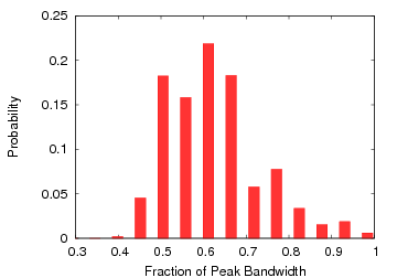 |
shows a visualisation of the histogram that resulted from 10000 simulation runs of the bidirectional bisection bandwidth measurement pattern, bisect_fb_sym, on a 16 node fat-tree with full bisection bandwidth. You can see the probability distribution for the bandwidth if a random mapping is simulated. It shows that full bisection bandwidth can be achieved, but only with a very small number of mappings, compared to the number of possible mappings.
The dep_max_delay metric is intended to be used together with the ptrnvsptrn communication pattern. This pattern merges two communication patterns by concatenating them. See the previous section for usage information for this pattern. This metric only examines the congestion in the first pattern, which is defined via the
--ptrnfst command line switch.
It simulates the whole pattern. Than it weights every edge in the communication
graph with the congestion factor of the route used for this communication. The
length (sum of the weights along the edges) of the longest path through the
communication graph is reported as the result. We call this number the
''delay'' the pattern experienced because of congestion. This yields a single
result for every simulation iteration. All delays are reported as a histogram
at the end of the simulation. By comparing the histogram of a simulation with a
pattern that uses the network to a histogram of a simulation with the null
pattern (as the second part of the pattern), the influence of the ''noise''
induced by the second pattern can be studied. The graph below
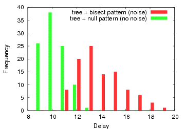 |
shows a visualization of the different histograms when this metric is used for 100 simulation runs of a tree pattern on 800 nodes of a 1142-host fat-tree network. The bisect pattern was used to generate ''noise'' on the rest of the hosts. In the noiseless case we utilized the null pattern. The graph shows how often a certain delay was observed in both cases.
The get_cong_map metrics aim is to help identifying bottlenecks in the network topology. After a simulation step is completed the cable congestion map contains the congestion factor for every edge that was used during this simulation step. With this metric the cable congestion map entries will be saved and further congestion entries, for the next level or simulation run, will be added. So after all simulation runs are finished we have recorded the sum of congestions that occurred over the entire simulation for every edge in the network topology graph. Edges that have never been used will have a congestion sum of zero. Then we will scale the congestion sums so that they become a number between zero and one by dividing them through the maximum of the recorded congestion sums. As a result this metric will print the network topology graph used as an input file, but every edge will be augmented with an additional property named, the scaled congestion sum. Also every edge will be given a color between green and red. The edges with the least relative congestion will be coloured in green, where the edges that have a comparatively high congestion sum will be coloured in red.
References
[1] T. Hoefler, T. Schneider and A. Lumsdaine:Multistage Switches are not Crossbars: Effects of Static Routing in High-Performance Networks In Proceedings of the 2008 IEEE International Conference on Cluster Computing, presented in Tsukuba, Japan, IEEE Computer Society, ISSN: 1552-5244, ISBN: 978-1-4244-2640, Oct. 2008[2] T. Hoefler>, T. Schneider and A. Lumsdaine:
[3] T. Schneider, T. Hoefler and A. Lumsdaine :ORCS: An Oblivious Routing Congestion Simulator Indiana University. Nr. 675, Indiana University Computer Science, Feb. 2009,
Download
Download the current version of ORCS:ORCS 1.1 - (57.33 kb)